A-10.7 Isomorphism between Polynomials and Vectors over Complex Numbers

In Theorem A-10.5 (§A-10.5), we learned the isomorphic mapping $\sigma :f(X)\in {\mathbb{Z}}_t[X]∕(X^n+1)\to (f(x_0),f(x_1),f(x_2),\cdots ,f(x_{n-1}))\in {\mathbb{Z}}_t^n$, where $x_0,x_1,x_2,\cdots ,x_{n-1}$ are the ($(\mu =2n)$-th primitive) roots of the cyclotomic polynomial $X^n+1$, which are $\omega ,{\omega }^3,{\omega }^5,\cdots ,{\omega }^{2n-1}$, where $\omega$ can be any root of $X^n+1$ (i.e., since each $\omega$ is a generator of all roots). In this subsection, we will demonstrate the isomorphism between a vector space and a polynomial ring over complex numbers as follows:

${\sigma }_c:f(X)\in ℝ[X]∕(X^n+1)\to (f(\omega ),f({\omega }^3),f({\omega }^5),\cdots ,f({\omega }^{2n-1}))\in {\widehat{ℂ}}^n$

, where $\omega =e^{\mathit{𝑖𝜋}∕n}$, the root (i.e., the primitive $(\mu =2n)$-th root) of the cyclotomic polynomial $X^n+1$ over complex numbers (Theorem A-8.2.1 in §A-8.2). We define ${\widehat{ℂ}}^n$ to be an $n$-dimensional special vector space whose second-half elements of each vector are reverse-ordered conjugates of the first-half elements (e.g., $(v_0,v_1,\cdots ,v_{\frac{n}{2}-1},{\overline{v}}_{\frac{n}{2}-1},\cdots ,{\overline{v}}_1,{\overline{v}}_0)$).

A-10.7.1 Isomorphism between ${ℂ}^{\frac{n}{2}}$ and ${\widehat{ℂ}}^n$

Bijective: Technically, ${\widehat{ℂ}}^n$ is bijective to ${ℂ}^{\frac{n}{2}}$, because the second-half $\frac{n}{2}$ elements of each vector in ${\widehat{ℂ}}^n$ are passively (automatically) determined by the first-half $\frac{n}{2}$ elements. Therefore, each vector in ${\widehat{ℂ}}^n$ has one-to-one correspondences with some unique vector in ${ℂ}^{\frac{n}{2}}$, and thus these two vector spaces are bijective.

Homomorphic: To demonstrate their homomorphism over the $\text{(+,⊙)}$ operations, we can apply the following reasoning: for all $\overrightarrow{\widehat{v}}\in {\widehat{ℂ}}^n$ and $\overrightarrow{v}\in {ℂ}^{\frac{n}{2}}$, there exists an ${\displaystyle \frac{n}{2}}\times n$ linear transformation matrix $M$ that satisfies $M\cdot \overrightarrow{\widehat{v}}=\overrightarrow{v}$. Such $M$ is an ${\displaystyle \frac{n}{2}}\times n$ matrix comprising horizontal concatenation of $I_{\frac{n}{2}}$ and ${[0]}_{\frac{n}{2}}$, where $I_{\frac{n}{2}}$ is an ${\displaystyle \frac{n}{2}}\times {\displaystyle \frac{n}{2}}$ identity matrix and ${[0]}_{\frac{n}{2}}$ is an ${\displaystyle \frac{n}{2}}\times {\displaystyle \frac{n}{2}}$ zero matrix. Also, there exists an $n\times {\displaystyle \frac{n}{2}}$ (non-linear) transformation matrix $N$ that satisfies $N\cdot \overrightarrow{v}=\overrightarrow{\widehat{v}}$. Such $N$ is a vertical concatenation of $I_{\frac{n}{2}}$ and ${\varnothing }_{\frac{n}{2}}^R$, where ${\varnothing }_{\frac{n}{2}}^R$ is an $\frac{n}{2}\times \frac{n}{2}$ matrix whose reverse-diagonal elements are unary conjugate operators and all other elements are zero. For example, if $n=4$, then $M$ and $N$ are structured as follows:

$M=\left[\begin{array}{cccccccc}\hfill 1\hfill & \hfill 0\hfill & \hfill 0\hfill & \hfill 0\hfill & \hfill 0\hfill & \hfill 0\hfill & \hfill 0\hfill & \hfill 0\hfill \\ \hfill 0\hfill & \hfill 1\hfill & \hfill 0\hfill & \hfill 0\hfill & \hfill 0\hfill & \hfill 0\hfill & \hfill 0\hfill & \hfill 0\hfill \\ \hfill 0\hfill & \hfill 0\hfill & \hfill 1\hfill & \hfill 0\hfill & \hfill 0\hfill & \hfill 0\hfill & \hfill 0\hfill & \hfill 0\hfill \\ \hfill 0\hfill & \hfill 0\hfill & \hfill 0\hfill & \hfill 1\hfill & \hfill 0\hfill & \hfill 0\hfill & \hfill 0\hfill & \hfill 0\hfill \end{array}\right]$, $N=\left[\begin{array}{cccc}\hfill 1\hfill & \hfill 0\hfill & \hfill 0\hfill & \hfill 0\hfill \\ \hfill 0\hfill & \hfill 1\hfill & \hfill 0\hfill & \hfill 0\hfill \\ \hfill 0\hfill & \hfill 0\hfill & \hfill 1\hfill & \hfill 0\hfill \\ \hfill 0\hfill & \hfill 0\hfill & \hfill 0\hfill & \hfill 1\hfill \\ \hfill 0\hfill & \hfill 0\hfill & \hfill 0\hfill & \hfill \varnothing \hfill \\ \hfill 0\hfill & \hfill 0\hfill & \hfill \varnothing \hfill & \hfill 0\hfill \\ \hfill 0\hfill & \hfill \varnothing \hfill & \hfill 0\hfill & \hfill 0\hfill \\ \hfill \varnothing \hfill & \hfill 0\hfill & \hfill 0\hfill & \hfill 0\hfill \end{array}\right]$

The reason $N$ is not a linear transformation matrix is because it contains conjugate operators $\varnothing$. Yet, notice that the following homomorphism holds between $\overrightarrow{\widehat{v}}\in {\widehat{ℂ}}^n$ and $\overrightarrow{v}\in {ℂ}^{\frac{n}{2}}$:

$N\cdot (M\cdot {\overrightarrow{\widehat{v}}}_1+M\cdot {\overrightarrow{\widehat{v}}}_2)={\overrightarrow{\widehat{v}}}_1+{\overrightarrow{\widehat{v}}}_2$, $M\cdot (N\cdot {\overrightarrow{v}}_1+N\cdot {\overrightarrow{v}}_2)={\overrightarrow{v}}_1+{\overrightarrow{v}}_2$

$N\cdot (M\cdot {\overrightarrow{\widehat{v}}}_1\odot M\cdot {\overrightarrow{\widehat{v}}}_2)={\overrightarrow{\widehat{v}}}_1\odot {\overrightarrow{\widehat{v}}}_2$, $M\cdot (N\cdot {\overrightarrow{v}}_1\odot N\cdot {\overrightarrow{v}}_2)={\overrightarrow{v}}_1\odot {\overrightarrow{v}}_2$

Thus, the ${\widehat{ℂ}}^n$ and ${ℂ}^{\frac{n}{2}}$ vector spaces are bijective and homomorphic over the $\text{(+,⊙)}$ operations, and therefore they preserve isomorphism.

A-10.7.2 Isomorphism between ${\widehat{ℂ}}^n$ and $ℝ[X]∕X^n+1$

Now, we will demonstrate ${\sigma }_c$’s isomorphism (i.e., bijective and homomorphic) between ${\widehat{ℂ}}^n$ and $ℝ[X]∕X^n+1$ by applying the same reasoning as described in the beginning of §A-10.6.

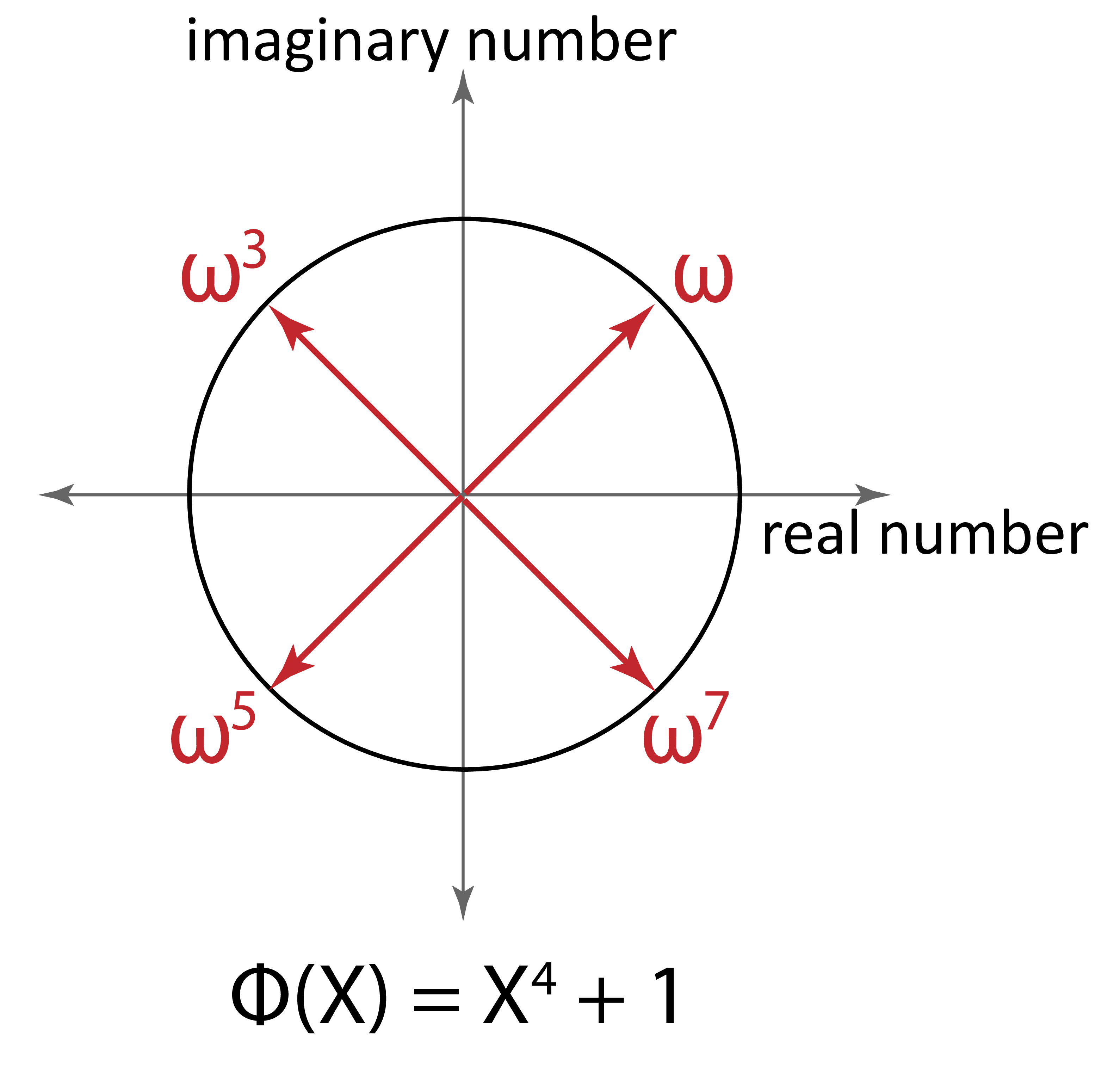
Bijective: Based on Euler’s formula $e^{\mathit{𝑖𝜃}}=\cos <!--\; FUNCTION\; APPLICATION\; -->𝜃+i\cdot \sin <!--\; FUNCTION\; APPLICATION\; -->𝜃$ (§A-11.3), we can derive the following arithmetic relations: $\omega =\overline{{\omega }^{2n-1}},{\omega }^3=\overline{{\omega }^{2n-3}},\cdots ,{\omega }^{n-1}=\overline{{\omega }^{n+1}}$. In other words, the one-half roots are conjugates of the other-half roots. This can also be pictorially understood based on a complex plane in Figure 5, where red arrows represent the roots of the 8th cyclotomic polynomial $X^4+1$, comprising imaginary number and real number components. As shown in this figure, one half of the red arrows (i.e., roots) are a reflection of the other half on the $x$-axis (i.e., imaginary number axis). This means that we can express these roots as an $n$-dimensional vector whose elements are the roots of $X^n+1$, such that its second-half elements are a reverse-ordered conjugate of the first-half elements. Based on this vector design, the $\sigma$ mapping can be re-written as follows:

$\sigma (f(X))=(f(\omega ),f({\omega }^3),f({\omega }^5),\cdots ,f({\omega }^{n-1}),f(\overline{{\omega }^{n-1}}),f(\overline{{\omega }^{n-3}}),\cdots ,f(\overline{{\omega }^3}),f(\overline{\omega }))$

Since $f(\overline{X})=\overline{f(X)}$, we can rewrite $\sigma$ as:

$\sigma (f(X))=(f(\omega ),f({\omega }^3),f({\omega }^5),\cdots ,f({\omega }^{n-3})f({\omega }^{n-1}),\overline{f({\omega }^{n-1})},\overline{f({\omega }^{n-3})},\cdots ,\overline{f({\omega }^3)},\overline{f(\omega ))}$

This structure of vector exactly aligns with the definition of ${\widehat{ℂ}}^n$: the first half of the elements of the $n$-dimensional vector $\overrightarrow{\widehat{v}}$ is a conjugate of the second half.

For bijectiveness, we also need to demonstrate that every $f(X)\in ℝ[X]∕X^n+1$ is mapped to some $\overrightarrow{\widehat{v}}\in {\widehat{ℂ}}^{\frac{n}{2}}$, and no two different $f_1(X),f_2(X)\in ℝ[X]∕X^n+1$ map to the same $\overrightarrow{\widehat{v}}\in {\widehat{ℂ}}^n$. The first requirement is satisfied because each polynomial $f(X)\in ℝ[X]∕X^n+1$ can be evaluated at the $n$ distinct roots of $X^n+1$ to a valid number. The second requirement is also satisfied because in the $(n-1)$-degree polynomial ring, each list of $n$ distinct $(x,y)$ coordinates (where we fix the $X$ values to the $n$ distinct roots of $X^2+1$ as $\{\omega ,{\omega }^3,\cdots ,{\omega }^{2n-1}\}$) can be mapped only to a single polynomial within the $(n-1)$-degree polynomial ring, as proved by Lagrange Polynomial Interpolation (Theorem A-15 in §A-15).

Homomorphic: ${\sigma }_c$ is homomorphic, because based on the reasoning shown in §A-10.6, the relations $\sigma (f_a(X)+f_b(X))=\sigma (f_a(X))+\sigma (f_b(X))$ and $\sigma (f_a(X)\cdot f_b(X))=\sigma (f_a(X))\odot \sigma (f_b(X))$ mathematically hold regardless of whether the type of $X$ is modulo integer or complex number,

Since ${\sigma }_c$ is both bijective and homomorphic over the $\text{(+,⋅)}$ operations, it is isomorphic.